Basic signal operation in DSP

In this article, we will discuss some basic signal operations, considering one of the signals as a constant value.

A signal can mathematically represent a change in a parameter.

If the value of the signal changes consistently with time, then we get an alternating signal. On the other hand, if the value of the signal remains constant over a wide range, then we get a signal with a constant value. These concepts are illustrated with alternating current (AC) and direct current (DC), respectively.

In this article, we will review the same basic signal operations as before but use constant value signals as examples.

Addition/subtraction of AC signals with constant value signals

Adding a signal: positive clamping

Let's start with the sinusoidal signal shown in the red curve in Figure 1.

Now, let's add a constant value signal with an amplitude of 1.5. Our output signal becomes y(t) = x(t) + 1.5. The blue curve represents the resulting plot in the same figure.

Figure 1. Summing the AC signal with a constant value of 1.5 in amplitude

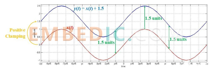
As you can see, y(t) is the same as x(t) but shifted by 1.5 amplitude along its trajectory (added to its constant value).

This is a good illustration of what happens when we add a constant value signal to an AC signal - the latter is shifted to the level of the former. This change in the reference level of the AC signal is called "clamping." Because, in this example, there is a shift to a positive value, we can call it "positive clamping."

What happens if we add the AC signal to a constant value signal? The mathematical equation would be y(t) = 1.5 + x(t).

However, the result will be the same. Why? As with simple math, addition is interchangeable, which means x(t) + 1.5 = 1.5 + x(t).

Subtractive signals: negative clamping

Next, let's try subtraction. We will start by subtracting our example constant-value signal from the AC signal. Let y(t) be x(t) - 1.5.

The output corresponding to this is the blue curve in Figure 2. By comparing this curve with the red curve representing the original signal, we can see that the signal's amplitude is reduced by 1.5 overall.

Figure 2. Effect of subtracting a constant value signal of 1.5 amplitude from the AC signal

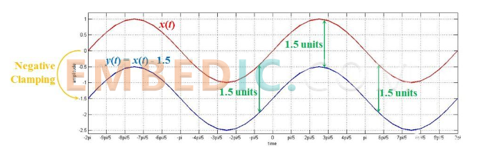
As it is clear from the figure, this has the direct effect of clamping the AC signal to -1.5. Since the clamping is towards the negative side, we call it "negative clamping."

When we write y(t) = x(t) - 1.5 as y(t) = - 1.5 + x(t), we can see that even in this case, the clamping must occur, but tends to be negative.

As a continuation, let us now try to reverse the order of the subtraction. That is, let our output signal be y(t) = 1.5 - x(t) instead of y(t) = x(t) - 1.5.

Figure 3 shows the results corresponding to this operation.

Figure 3. Effect of subtracting the AC signal from a constant-value signal with an amplitude of 1.5

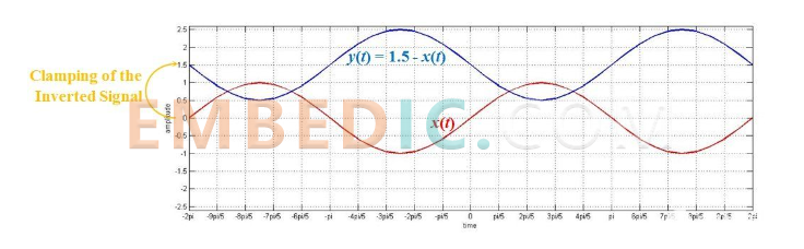
At first glance, this seems to throw the idea of "clamping" out the window. However, this is not entirely true.

Why?

Look closely. The blue curve in the graph is the alternating signal but reversed along the horizontal axis and clamped at the 1.5 level.

In this case, our output equation is y(t) = 1.5 - x(t), which is the same as y(t) = 1.5 + {-x(t)}. This indicates that the inverted x(t) should be restricted to the level of 1.5 in this case.

Conclusion on addition or subtraction

We can conclude that adding or subtracting a constant-valued signal to an alternating signal always clamps the alternating signal to a value determined by a constant.

In electronic terms, the circuit that generates the clamp is called a "clamp."

So we know that addition/subtraction operations performed on signals where at least one of them is a constant value can find their use in all scenarios where a clamp is applied. Baseline stabilizers, DC recovery circuits, and circuits used to establish compatibility between the device's operating range and the input signal's operating range are just a few examples of applications where you might see these operations.

The effect of multiplying a constant value signal with an AC signal

In this section, we will study the effect of multiplying a constant value signal with an alternating signal. In particular, let us multiply a constant-valued signal of amplitude 1.5 with an alternating signal x(t), which is a sine wave of period 2π (as shown by the red curve in Figure 4).

The resulting plot is shown as a blue curve in Figure 4.

Figure 4. Constant value signal with an amplitude of 1.5 multiplied by AC signal

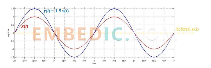
As can be seen in the figure, x(t) has a value of -1 at -π/2, and y(t) has a value of -1.5 (i.e., 1.5 times the value of x(t)). Similarly, at moments 0, π/2, and 3π/2, we have y(t) values of 0, 1.5, and -1.5, respectively, and you will notice that these are the values of x(t) (0, 1, and -1, respectively) multiplied by 1.5.

This shows that when we multiply a signal by a constant value, we get a signal whose value is multiplied by the same factor.

At this point, we should discuss an important point related to Figure 4. Unlike addition and subtraction (as shown in Figures 1 through 3), multiplication does not result in signal clamping. However, as with addition, multiplication is exchangeable, giving y(t) = 1.5 x(t) = x(t) 1.5.

Conclusion on multiplication

It is clear from the above discussion that multiplying a signal with a constant greater than 1 increases its amplitude without clamping it. This essentially amplifies the input signal by a factor determined by the value of the constant. Therefore, this multiplication operation is useful in all cases where electronic amplifiers are used.

Some examples of this are low-noise amplifiers in communication systems, audio/video amplifiers for radio/TV sets, and operational amplifiers that form an integral part of numerous electronic circuits.

Differentiation and integration of constant-valued signals

According to mathematics, the differentiation of a constant will be zero. This is true even in the case of signals. By differentiating a constant-valued signal, we will get a zero-valued signal. This is the working principle behind the work of the isolation capacitors used in many electronic designs.

On the other hand, if we integrate a constant value signal, we will get a slope whose slope is determined by the constant value. Circuits like constant current ramp generators work according to this principle.

Overview

In this article, we analyzed the results of applying a constant value signal to a basic signal operation. We also saw how operations such as addition/subtraction, multiplication, differentiation, and integration produce effects such as clamping, amplification, DC blocking, and ramp generation, respectively.